More logging

Germany was great. The Max Planck Institute for Math is an incredible place to do research, from the wonderful staff to the good talks to the coffee machine on the main floor. My collaborator and I made a lot of progress and I learned a lot about the affine Grassmannian. Maybe pictures to follow.

I had a good jetlag-free week in Germany and then came back to the US and got into the work rhythm again. Side projects: Am I ready for college math? Trying to figure out how to provide good resources to students to deal with the psychological side of math, since I see so many students drop out because of feelings rather than ability. I put up my first Youtube video on stereotype threat while in Germany. Just putting it together was interesting! The next set of videos will probably be shorter…. Work projects: I’m leading a seminar on CCAR and stress testing. CCAR stands for “Comprehensive Capital Analysis and Review,” and it’s a process in which banks have to justify to the Federal Reserve that they’ve got enough money to deal with their obligations should the economic situation get bad. It’s directly in response to the financial crisis of the late 2000s and there is a TON of math modeling involved.

Next week I’ll be helping with the math modeling workshop for high school students at the University of Minnesota, and my group will be working on nitrate runoff in southern Minnesota. Prepping for that has been interesting — it’s math and nature (so related to a lot of activities I’ve written up for Earthcalculus.com) but there are some definite financial aspects, too. Finance and risk management in agriculture are going to be a theme in the Actuarial Research Conference that MCFAM is organizing at the University of Minnesota and St Thomas this summer!

Also trying to keep up with the weeds in the back yard…. things grow so fast!!! Our corn is showing tassels already (new fertilizer regimen) and we’ve got strawberries galore…. The hops are growing like crazy and we’ll have a good crop this year.
Putting the log in blog again

Finals week and life lessons

Asking to do work to bring up your score after the final is like putting on makeup after the party.

We make a link in school between doing work and getting points that enable one to pass a class, but maybe I need to remember how to emphasize that doing good work is the important thing, not just making an effort. Putting in the time is extraordinarily important, but in the end we’re measured on results, rather than effort.

In any long-term project it’s better to focus on effort in the short term, because results don’t emerge for so long. But it doesn’t make the results irrelevant. They are still the point in many cases.

Interesting to meditate on as I spend a research-focused two weeks after grading a lot of finals.

Germany

I got some beer & honey organic shampoo. Smells nice. Seems a good way to start the day.

I am so jetlagged it is ridiculous. Up at 3 am, back to “sleep” 5-7 am. Then yoga & exercise and soon to work. An espresso will start things off right but I might need an afternoon nap. I know people say that naps are counterproductive but 5 hrs sleep kills me and migraines are not conducive to mathematical genius.

I can’t manage trash here. I understand that all trash needs to be sorted into blue, yellow, and black bins — but where are these bins?!

Lots of chocolate shops here. Delightful.

TDAmapper in R

Today I finally checked out the R package TDAmapper. I found very few tutorials for it, so here’s a bit of discussion

Curiously, there’s a lot more discussion of the math out there than the implementation. I just found Chad Topaz’s “Self-Help Homology Tutorial for the Simple(x)-minded” at his website, and there’s a more technical intro by Elizabeth Munch, and you can look up Ayasdi videos on YouTube for plenty more options — Ayasdi is the company started by Stanford math prof Gunnar Carlsson and others to try to use this mathematics for commercial purposes.

I’m going to just start with the examples in the TDAmapper documentation, though, as I understand the math reasonably well but have tons of questions about implementation that aren’t extensively discussed. Let’s get started!

mapper1D

Quoting from the documentation,

mapper1D(distance_matrix = dist(data.frame(x = 2 * cos(0.5 * (1:100)), y = sin(1:100))), filter_values = 2 * cos(0.5 * (1:100)), num_intervals = 10,
percent_overlap = 50, num_bins_when_clustering = 10)

What’s going on here?

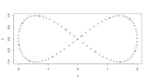
We’ve got data, which here is this cute artificial set in the shape of a infinity symbol:

plot(data.frame(x=2*cos(0.5*(1:100)), y=sin(1:100))) 
InfinitySymbol

gives an illustration.

Continue reading

Random walks in Python

I’ve been finishing up the semester and talking about random walks and Brownian motion. In order to add some images to my course notes at https://www.softcover.io/read/bf34ea25/math_for_finance, I made some quick Python calculations:

Simple symmetric random walk: The laziest thing I could think of was to use the binomial function from numpy. It returns 0 or 1, so I simply translated it (x->2x-1) so that I can get 1 or -1 instead.

from math import sqrt
import numpy as np
import matplotlib.pyplot as plt
%matplotlib inline

def RandomWalk(N,d):
walk = np.cumsum(2*np.random.binomial(1,.5,N)-1)
return walk

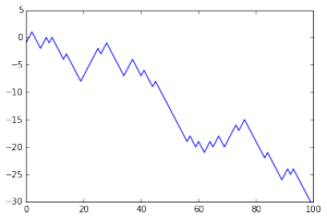
It’s easy then to plot this:

plt.plot(np.arange(100),RandomWalk(100,1))
plt.show()

OneRandomWalk

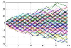
Of course, rather than looking at one random walk, it’s more fun to look at a bunch. Here’s 180 simple symmetric random walks:

RandomWalks

I plotted this using the following code:

endpoints = []
for k in range(180):
particularWalk = RandomWalk(100,1)
endpoints.append(particularWalk[-1])
plt.plot(np.arange(100),particularWalk)
grid(True)
plt.show()

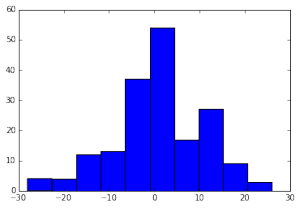
This also peeled off the endpoints of the walks (at step 100), so that I could make a histogram of the positions at time 100:

HistogramOfEndpoints

The idea is to show the distribution of S_100, position at time 100. We know that as n goes to infinity we can say that the limiting distribution for S_n is the normal distribution; 100 is quite far from infinity but even there we start getting some idea of the distribution.

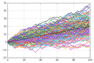
I also generated some asymmetrical simple random walks — still one step of length 1 each time unit, but now one direction is more probable than the other:

AsymmRandomWalk.6

This above is a random walk with P(X=1) = 0.6 and P(X=-1)=0.4. The expected value is plotted with the black line on top.

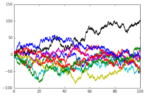
And last, I showed what horrible things can happen if you scale time (taking steps in the random walk more quickly) without scaling time:

TooManySteps

The variance goes crazy (not that I showed that) and the character of the walks seems to change. Yes, that’s touchy-feely talk, but I want people to have a feeling for the shape of Brownian motion. I’ll put some of that up later!